| pix2pix:使用条件 GAN 进行图像到图像的转换 | 您所在的位置:网站首页 › gan 损失函数 › pix2pix:使用条件 GAN 进行图像到图像的转换 |
pix2pix:使用条件 GAN 进行图像到图像的转换
 在 GitHub 上查看源代码 在 GitHub 上查看源代码
本教程演示了如何构建和训练一个名为 pix2pix 的条件生成对抗网络 (cGAN),该网络学习从输入图像到输出图像的映射,如 Isola 等人在 Image-to-image translation with conditional adversarial networks (2017 年)中所述 。pix2pix 非特定于应用,它可以应用于多种任务,包括从标签地图合成照片,从黑白图像生成彩色照片,将 Google Maps 照片转换为航拍图像,甚至将草图转换为照片。 在此示例中,您的网络将使用布拉格捷克理工大学的机器感知中心提供的 CMP Facade Database 来生成建筑立面。为了简化示例,您将使用由 pix2pix 作者创建的此数据集的预处理副本。 在 pix2pix cGAN 中,您可以对输入图像进行调节并生成相应的输出图像。cGAN 最初在 Conditional Generative Adversarial Nets (Mirza and Osindero, 2014) 中提出。 您的网络架构将包含: 基于 U-Net 架构的生成器。 由卷积 PatchGAN 分类器表示的判别器(在 pix2pix 论文中提出)。请注意,在单个 V100 GPU 上,每个周期可能需要大约 15 秒。 以下是 pix2pix cGAN 在 Facade Database(8 万步)上训练 200 个周期后生成的一些输出示例。
下载 CMP Facade Database 数据 (30MB)。可在这里以相同格式获得其他数据集。在 Colab 中,您可以从下拉菜单中选择其他数据集。请注意,其他一些数据集要大得多(edges2handbags 为 8GB)。 dataset_name = "facades" _URL = f'http://efrosgans.eecs.berkeley.edu/pix2pix/datasets/{dataset_name}.tar.gz' path_to_zip = tf.keras.utils.get_file( fname=f"{dataset_name}.tar.gz", origin=_URL, extract=True) path_to_zip = pathlib.Path(path_to_zip) PATH = path_to_zip.parent/dataset_name Downloading data from http://efrosgans.eecs.berkeley.edu/pix2pix/datasets/facades.tar.gz 30168306/30168306 [==============================] - 13s 0us/step list(PATH.parent.iterdir()) [PosixPath('/home/kbuilder/.keras/datasets/iris_training.csv'), PosixPath('/home/kbuilder/.keras/datasets/facades.tar.gz'), PosixPath('/home/kbuilder/.keras/datasets/facades'), PosixPath('/home/kbuilder/.keras/datasets/iris_test.csv'), PosixPath('/home/kbuilder/.keras/datasets/YellowLabradorLooking_new.jpg'), PosixPath('/home/kbuilder/.keras/datasets/kandinsky5.jpg'), PosixPath('/home/kbuilder/.keras/datasets/mnist.npz'), PosixPath('/home/kbuilder/.keras/datasets/fashion-mnist')]每个原始图像的大小为 256 x 512,包含两个 256 x 256 图像: sample_image = tf.io.read_file(str(PATH / 'train/1.jpg')) sample_image = tf.io.decode_jpeg(sample_image) print(sample_image.shape) (256, 512, 3) plt.figure() plt.imshow(sample_image)
您需要将真实的建筑立面图像与建筑标签图像分开,所有这些图像的大小都是 256 x 256。 定义加载图像文件并输出两个图像张量的函数: def load(image_file): # Read and decode an image file to a uint8 tensor image = tf.io.read_file(image_file) image = tf.io.decode_jpeg(image) # Split each image tensor into two tensors: # - one with a real building facade image # - one with an architecture label image w = tf.shape(image)[1] w = w // 2 input_image = image[:, w:, :] real_image = image[:, :w, :] # Convert both images to float32 tensors input_image = tf.cast(input_image, tf.float32) real_image = tf.cast(real_image, tf.float32) return input_image, real_image绘制输入图像(建筑标签图像)和真实(建筑立面照片)图像的样本: inp, re = load(str(PATH / 'train/100.jpg')) # Casting to int for matplotlib to display the images plt.figure() plt.imshow(inp / 255.0) plt.figure() plt.imshow(re / 255.0)
如 pix2pix 论文中所述,您需要应用随机抖动和镜像来预处理训练集。 定义几个具有以下功能的函数: 将每个 256 x 256 图像调整为更大的高度和宽度,286 x 286。 将其随机裁剪回 256 x 256。 随机水平翻转图像,即从左到右(随机镜像)。 将图像归一化到 [-1, 1] 范围。 # The facade training set consist of 400 images BUFFER_SIZE = 400 # The batch size of 1 produced better results for the U-Net in the original pix2pix experiment BATCH_SIZE = 1 # Each image is 256x256 in size IMG_WIDTH = 256 IMG_HEIGHT = 256 def resize(input_image, real_image, height, width): input_image = tf.image.resize(input_image, [height, width], method=tf.image.ResizeMethod.NEAREST_NEIGHBOR) real_image = tf.image.resize(real_image, [height, width], method=tf.image.ResizeMethod.NEAREST_NEIGHBOR) return input_image, real_image def random_crop(input_image, real_image): stacked_image = tf.stack([input_image, real_image], axis=0) cropped_image = tf.image.random_crop( stacked_image, size=[2, IMG_HEIGHT, IMG_WIDTH, 3]) return cropped_image[0], cropped_image[1] # Normalizing the images to [-1, 1] def normalize(input_image, real_image): input_image = (input_image / 127.5) - 1 real_image = (real_image / 127.5) - 1 return input_image, real_image @tf.function() def random_jitter(input_image, real_image): # Resizing to 286x286 input_image, real_image = resize(input_image, real_image, 286, 286) # Random cropping back to 256x256 input_image, real_image = random_crop(input_image, real_image) if tf.random.uniform(()) > 0.5: # Random mirroring input_image = tf.image.flip_left_right(input_image) real_image = tf.image.flip_left_right(real_image) return input_image, real_image您可以检查部分预处理输出: plt.figure(figsize=(6, 6)) for i in range(4): rj_inp, rj_re = random_jitter(inp, re) plt.subplot(2, 2, i + 1) plt.imshow(rj_inp / 255.0) plt.axis('off') plt.show()
检查加载和预处理能够正常工作后,我们来定义两个辅助函数来加载和预处理训练集和测试集: def load_image_train(image_file): input_image, real_image = load(image_file) input_image, real_image = random_jitter(input_image, real_image) input_image, real_image = normalize(input_image, real_image) return input_image, real_image def load_image_test(image_file): input_image, real_image = load(image_file) input_image, real_image = resize(input_image, real_image, IMG_HEIGHT, IMG_WIDTH) input_image, real_image = normalize(input_image, real_image) return input_image, real_image 使用 tf.data 构建输入流水线 train_dataset = tf.data.Dataset.list_files(str(PATH / 'train/*.jpg')) train_dataset = train_dataset.map(load_image_train, num_parallel_calls=tf.data.AUTOTUNE) train_dataset = train_dataset.shuffle(BUFFER_SIZE) train_dataset = train_dataset.batch(BATCH_SIZE) try: test_dataset = tf.data.Dataset.list_files(str(PATH / 'test/*.jpg')) except tf.errors.InvalidArgumentError: test_dataset = tf.data.Dataset.list_files(str(PATH / 'val/*.jpg')) test_dataset = test_dataset.map(load_image_test) test_dataset = test_dataset.batch(BATCH_SIZE) 构建生成器您的 pix2pix cGAN 是经过修改的 U-Net。U-Net 由编码器(下采样器)和解码器(上采样器)。(有关详细信息,请参阅图像分割教程和 U-Net 项目网站。) 编码器中的每个块为:Convolution -> Batch normalization -> Leaky ReLU 解码器中的每个块为:Transposed convolution -> Batch normalization -> Dropout(应用于前三个块)-> ReLU 编码器和解码器之间存在跳跃连接(如在 U-Net 中)。定义下采样器(编码器): OUTPUT_CHANNELS = 3 def downsample(filters, size, apply_batchnorm=True): initializer = tf.random_normal_initializer(0., 0.02) result = tf.keras.Sequential() result.add( tf.keras.layers.Conv2D(filters, size, strides=2, padding='same', kernel_initializer=initializer, use_bias=False)) if apply_batchnorm: result.add(tf.keras.layers.BatchNormalization()) result.add(tf.keras.layers.LeakyReLU()) return result down_model = downsample(3, 4) down_result = down_model(tf.expand_dims(inp, 0)) print (down_result.shape) (1, 128, 128, 3)定义上采样器(解码器): def upsample(filters, size, apply_dropout=False): initializer = tf.random_normal_initializer(0., 0.02) result = tf.keras.Sequential() result.add( tf.keras.layers.Conv2DTranspose(filters, size, strides=2, padding='same', kernel_initializer=initializer, use_bias=False)) result.add(tf.keras.layers.BatchNormalization()) if apply_dropout: result.add(tf.keras.layers.Dropout(0.5)) result.add(tf.keras.layers.ReLU()) return result up_model = upsample(3, 4) up_result = up_model(down_result) print (up_result.shape) (1, 256, 256, 3)使用下采样器和上采样器定义生成器: def Generator(): inputs = tf.keras.layers.Input(shape=[256, 256, 3]) down_stack = [ downsample(64, 4, apply_batchnorm=False), # (batch_size, 128, 128, 64) downsample(128, 4), # (batch_size, 64, 64, 128) downsample(256, 4), # (batch_size, 32, 32, 256) downsample(512, 4), # (batch_size, 16, 16, 512) downsample(512, 4), # (batch_size, 8, 8, 512) downsample(512, 4), # (batch_size, 4, 4, 512) downsample(512, 4), # (batch_size, 2, 2, 512) downsample(512, 4), # (batch_size, 1, 1, 512) ] up_stack = [ upsample(512, 4, apply_dropout=True), # (batch_size, 2, 2, 1024) upsample(512, 4, apply_dropout=True), # (batch_size, 4, 4, 1024) upsample(512, 4, apply_dropout=True), # (batch_size, 8, 8, 1024) upsample(512, 4), # (batch_size, 16, 16, 1024) upsample(256, 4), # (batch_size, 32, 32, 512) upsample(128, 4), # (batch_size, 64, 64, 256) upsample(64, 4), # (batch_size, 128, 128, 128) ] initializer = tf.random_normal_initializer(0., 0.02) last = tf.keras.layers.Conv2DTranspose(OUTPUT_CHANNELS, 4, strides=2, padding='same', kernel_initializer=initializer, activation='tanh') # (batch_size, 256, 256, 3) x = inputs # Downsampling through the model skips = [] for down in down_stack: x = down(x) skips.append(x) skips = reversed(skips[:-1]) # Upsampling and establishing the skip connections for up, skip in zip(up_stack, skips): x = up(x) x = tf.keras.layers.Concatenate()([x, skip]) x = last(x) return tf.keras.Model(inputs=inputs, outputs=x)可视化生成器模型架构: generator = Generator() tf.keras.utils.plot_model(generator, show_shapes=True, dpi=64)
测试生成器: gen_output = generator(inp[tf.newaxis, ...], training=False) plt.imshow(gen_output[0, ...]) Clipping input data to the valid range for imshow with RGB data ([0..1] for floats or [0..255] for integers).
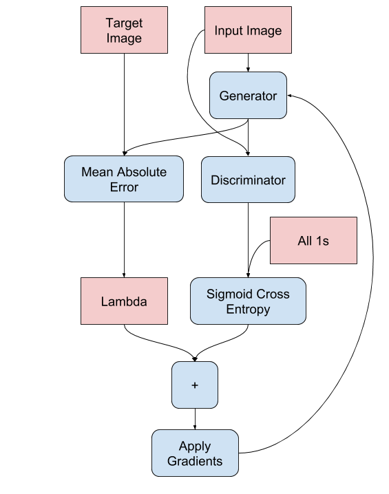
GAN 学习适应数据的损失,而 cGAN 学习结构化损失,该损失会惩罚与网络输出和目标图像不同的可能结构,如 pix2pix 论文中所述。 生成器损失是生成图像和一数组的 sigmoid 交叉熵损失。 论文还提到了 L1 损失,它是生成图像与目标图像之间的 MAE(平均绝对误差)。 这样可使生成的图像在结构上与目标图像相似。 计算总生成器损失的公式为:gan_loss + LAMBDA * l1_loss,其中 LAMBDA = 100。该值由论文作者决定。 LAMBDA = 100 loss_object = tf.keras.losses.BinaryCrossentropy(from_logits=True) def generator_loss(disc_generated_output, gen_output, target): gan_loss = loss_object(tf.ones_like(disc_generated_output), disc_generated_output) # Mean absolute error l1_loss = tf.reduce_mean(tf.abs(target - gen_output)) total_gen_loss = gan_loss + (LAMBDA * l1_loss) return total_gen_loss, gan_loss, l1_loss生成器的训练过程如下:
pix2pix cGAN 中的判别器是一个卷积 PatchGAN 分类器,它会尝试对每个图像分块的真实与否进行分类,如 pix2pix 论文中所述。 判别器中的每个块为:Convolution -> Batch normalization -> Leaky ReLU。 最后一层之后的输出形状为 (batch_size, 30, 30, 1)。 输出的每个 30 x 30 图像分块会对输入图像的 70 x 70 部分进行分类。 判别器接收 2 个输入: 输入图像和目标图像,应分类为真实图像。 输入图像和生成图像(生成器的输出),应分类为伪图像。 使用tf.concat([inp, tar], axis=-1) 将这 2 个输入连接在一起。我们来定义判别器: def Discriminator(): initializer = tf.random_normal_initializer(0., 0.02) inp = tf.keras.layers.Input(shape=[256, 256, 3], name='input_image') tar = tf.keras.layers.Input(shape=[256, 256, 3], name='target_image') x = tf.keras.layers.concatenate([inp, tar]) # (batch_size, 256, 256, channels*2) down1 = downsample(64, 4, False)(x) # (batch_size, 128, 128, 64) down2 = downsample(128, 4)(down1) # (batch_size, 64, 64, 128) down3 = downsample(256, 4)(down2) # (batch_size, 32, 32, 256) zero_pad1 = tf.keras.layers.ZeroPadding2D()(down3) # (batch_size, 34, 34, 256) conv = tf.keras.layers.Conv2D(512, 4, strides=1, kernel_initializer=initializer, use_bias=False)(zero_pad1) # (batch_size, 31, 31, 512) batchnorm1 = tf.keras.layers.BatchNormalization()(conv) leaky_relu = tf.keras.layers.LeakyReLU()(batchnorm1) zero_pad2 = tf.keras.layers.ZeroPadding2D()(leaky_relu) # (batch_size, 33, 33, 512) last = tf.keras.layers.Conv2D(1, 4, strides=1, kernel_initializer=initializer)(zero_pad2) # (batch_size, 30, 30, 1) return tf.keras.Model(inputs=[inp, tar], outputs=last)可视化判别器模型架构: discriminator = Discriminator() tf.keras.utils.plot_model(discriminator, show_shapes=True, dpi=64)
测试判别器: disc_out = discriminator([inp[tf.newaxis, ...], gen_output], training=False) plt.imshow(disc_out[0, ..., -1], vmin=-20, vmax=20, cmap='RdBu_r') plt.colorbar()
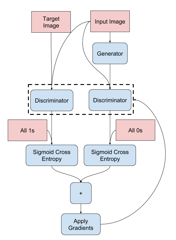
判别器的训练过程如下所示。 要详细了解架构和超参数,请参阅 pix2pix 论文。
编写函数以在训练期间绘制一些图像。 将图像从测试集传递到生成器。 然后,生成器会将输入图像转换为输出。 最后一步是绘制预测,瞧!注:在这里,training=True 是有意的,因为在基于测试数据集运行模型时,您需要批次统计信息。如果您使用 training = False,将获得从训练数据集中学习的累积统计信息(您不需要)。 def generate_images(model, test_input, tar): prediction = model(test_input, training=True) plt.figure(figsize=(15, 15)) display_list = [test_input[0], tar[0], prediction[0]] title = ['Input Image', 'Ground Truth', 'Predicted Image'] for i in range(3): plt.subplot(1, 3, i+1) plt.title(title[i]) # Getting the pixel values in the [0, 1] range to plot. plt.imshow(display_list[i] * 0.5 + 0.5) plt.axis('off') plt.show()测试该函数: for example_input, example_target in test_dataset.take(1): generate_images(generator, example_input, example_target)
实际的训练循环。由于本教程可以运行多个数据集,并且数据集的大小差异很大,因此将训练循环设置为按步骤而非按周期工作。 迭代步骤数。 每 10 步打印一个点 (.)。 每 1 千步:清除显示并运行 generate_images 以显示进度。 每 5 千步:保存一个检查点。 def fit(train_ds, test_ds, steps): example_input, example_target = next(iter(test_ds.take(1))) start = time.time() for step, (input_image, target) in train_ds.repeat().take(steps).enumerate(): if (step) % 1000 == 0: display.clear_output(wait=True) if step != 0: print(f'Time taken for 1000 steps: {time.time()-start:.2f} sec\n') start = time.time() generate_images(generator, example_input, example_target) print(f"Step: {step//1000}k") train_step(input_image, target, step) # Training step if (step+1) % 10 == 0: print('.', end='', flush=True) # Save (checkpoint) the model every 5k steps if (step + 1) % 5000 == 0: checkpoint.save(file_prefix=checkpoint_prefix)此训练循环会保存日志,您可以在 TensorBoard 中查看这些日志以监控训练进度。 如果您使用的是本地计算机,则需要启动一个单独的 TensorBoard 进程。在笔记本中工作时,请在开始训练之前启动查看器以使用 TensorBoard 进行监控。 To launch the viewer paste the following into a code-cell: %load_ext tensorboard %tensorboard --logdir {log_dir}最后,运行训练循环: fit(train_dataset, test_dataset, steps=40000) Time taken for 1000 steps: 92.81 sec
如果要公开共享 TensorBoard 结果,可以通过将以下代码复制到代码单元中的方式将日志上传到 TensorBoard.dev。 注:此操作需要一个 Google 帐号。 tensorboard dev upload --logdir {log_dir}小心:此命令不会终止。它可以连续上传长时间运行实验的结果。数据上传后,您需要使用笔记本工具中的“Interrupt Execution”选项将其停止。 您可以在 TensorBoard.dev 上查看此笔记本先前运行的结果。 TensorBoard.dev 是一种托管式体验,用于托管、跟踪机器学习实验并与所有人共享。 也可以使用 将其包含在行内: display.IFrame( src="https://tensorboard.dev/experiment/lZ0C6FONROaUMfjYkVyJqw", width="100%", height="1000px")与简单的分类或回归模型相比,在训练 GAN(或像 pix2pix 这样的 cGAN)时,对日志的解释更加微妙。要检查的内容包括: 检查生成器模型或判别器模型均未“获胜”。如果 gen_gan_loss 或 disc_loss 变得很低,则表明此模型正在支配另一个模型,并且您未能成功训练组合模型。 值 log(2) = 0.69 是这些损失的一个良好参考点,因为它表示困惑度为 2:判别器对这两个选项的平均不确定性是相等的。 对于 disc_loss,低于 0.69 的值意味着判别器在真实图像和生成图像的组合集上的表现要优于随机数。 对于 gen_gan_loss,如果值小于 0.69,则表示生成器在欺骗判别器方面的表现要优于随机数。 随着训练的进行,gen_l1_loss 应当下降。 恢复最新的检查点并测试网络 ls {checkpoint_dir} checkpoint ckpt-5.data-00000-of-00001 ckpt-1.data-00000-of-00001 ckpt-5.index ckpt-1.index ckpt-6.data-00000-of-00001 ckpt-2.data-00000-of-00001 ckpt-6.index ckpt-2.index ckpt-7.data-00000-of-00001 ckpt-3.data-00000-of-00001 ckpt-7.index ckpt-3.index ckpt-8.data-00000-of-00001 ckpt-4.data-00000-of-00001 ckpt-8.index ckpt-4.index # Restoring the latest checkpoint in checkpoint_dir checkpoint.restore(tf.train.latest_checkpoint(checkpoint_dir)) 使用测试集生成一些图像 # Run the trained model on a few examples from the test set for inp, tar in test_dataset.take(5): generate_images(generator, inp, tar)
|


【本文地址】